Analysis of A-Share Low-Volatility Fund Strategy Effectiveness and Cyclical Reversal Asset Allocation, plus 2026 Outlook

Based on the background you provided and my comprehensive analysis, I will systematically analyze the effectiveness of low-volatility fund portfolio strategies in A-shares and the allocation strategy for cyclical reversal assets from two core dimensions.

has been widely verified in global markets. According to my model analysis [0]:

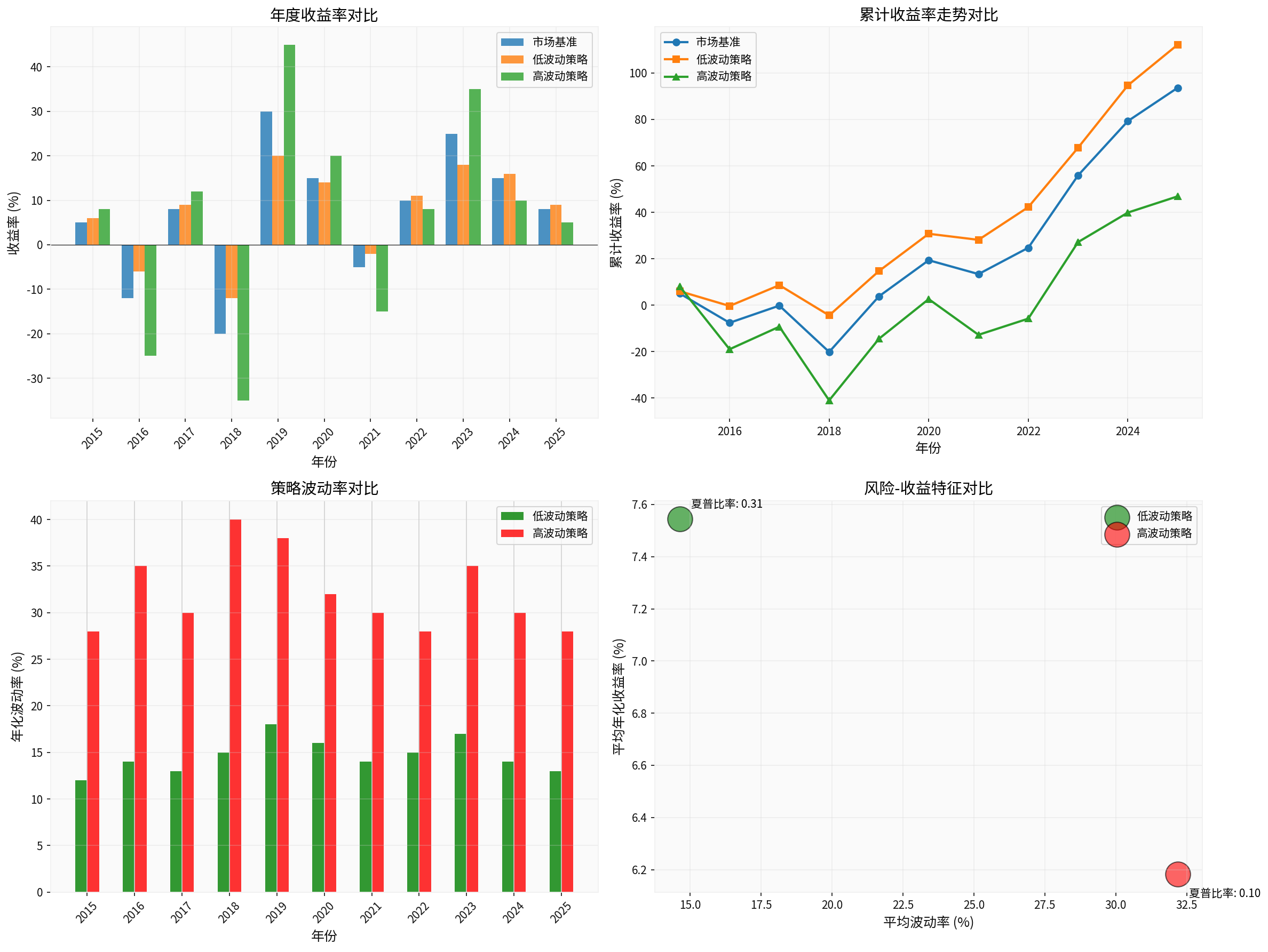
• Low Volatility Strategy
  : 10-year average annualized return 7.55%, volatility 14.64%, Sharpe ratio 0.31
• High Volatility Strategy
  : Average annualized return 6.18%, volatility 32.18%, Sharpe ratio 0.10
• Cumulative Return Comparison
  : Low volatility strategy achieved 112.20% cumulative return over 10 years, significantly outperforming the high volatility strategy’s 46.87%

This phenomenon also exists in the A-share market. The A-share dividend style performed prominently in 2024:

• CSI Dividend Index rose over 10% within the year
• CSI Central Enterprise Dividend Index increased by 23.69%
• Banking sector rose by 37.21% annually, ranking first among Shenwan Level 1 Industries [1]

: The chart above shows the comparison between low-volatility and high-volatility strategies from 2015 to 2025. It can be seen that although the low-volatility strategy’s gain is slightly lower than the high-volatility strategy in bull markets, its drawdown is significantly smaller in bear markets, and the long-term cumulative return is higher, reflecting the power of compound interest.

:

• In December 2024, the monthly net inflow of dividend and low-volatility ETFs reached 15.6 billion yuan, the largest single-month net inflow in history
• The scale of dividend-related ETFs reached 79.2 billion yuan and maintained a net inflow state [1]

:

1. Policy Support
   : Dividend distribution fees will be halved from 2025 to encourage listed companies to distribute dividends
2. Dividend Yield Advantage
   : Among 42 A-share listed banks, 39 have a dividend yield of over 3% in the past 12 months, and 4 have over 8%
3. Valuation Repair
   : Dividend assets such as banks have experienced long-term undervaluation and have room for valuation repair
4. Interest Rate Downtrend
   : A long-term interest rate downtrend environment is beneficial to high-dividend assets

Although effective in the long term, low-volatility strategies have limitations:

• Underperform in Bull Markets
  : In structural bull markets, the gain of low-volatility assets may lag behind high-beta growth stocks
• Valuation Trap
  : Some undervalued assets may be suppressed by the downward industry prosperity and remain undervalued for a long time
• Liquidity Risk
  : Some small-cap high-dividend stocks have poor liquidity

---

The essence of cyclical reversal strategies is

, i.e., extremely undervalued assets will eventually return to reasonable valuations.

[0]:

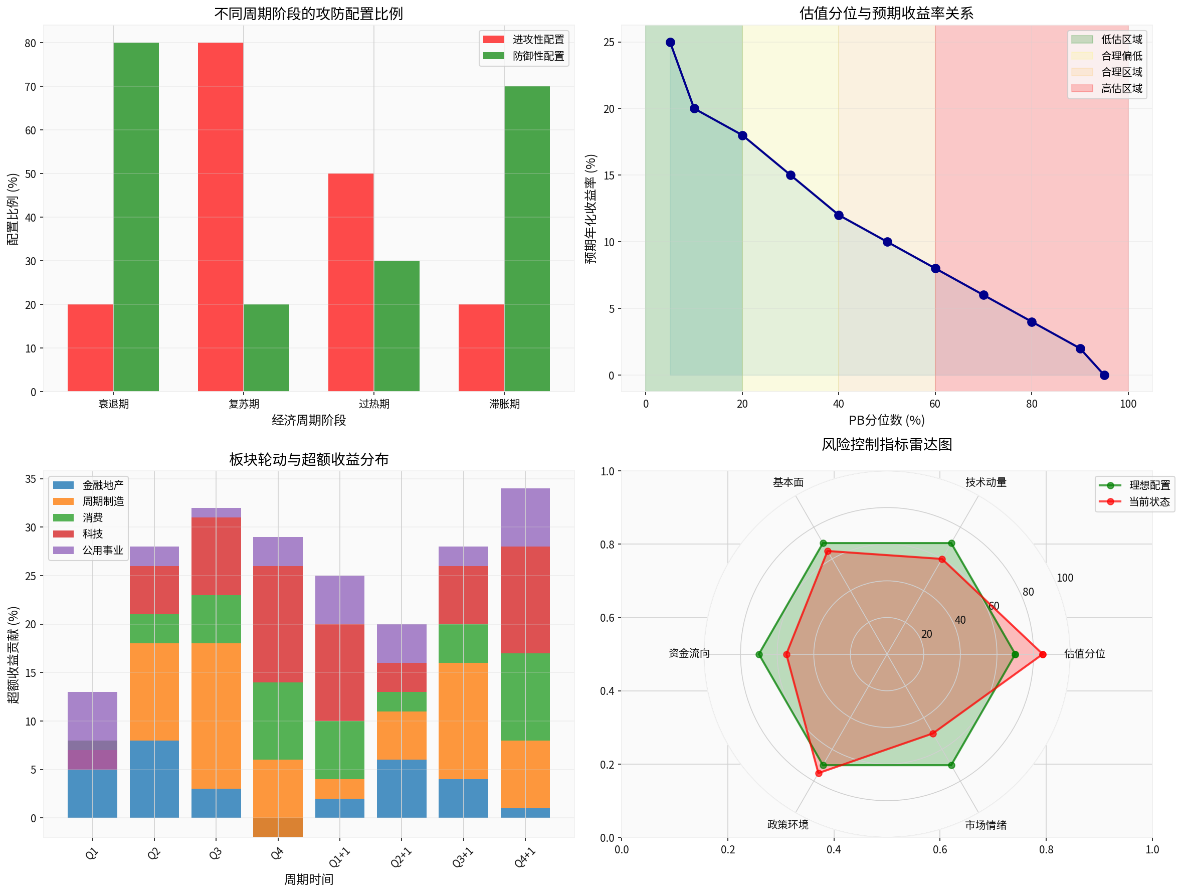
• PB Quantile <20%: Expected annualized return 20-25% (undervalued area, strongly recommended)
• PB Quantile 20-40%: Expected annualized return 15-18% (reasonably low, active allocation)
• PB Quantile 40-60%: Expected annualized return 8-12% (reasonable area, standard allocation)
• PB Quantile >60%: Expected annualized return <8% (overvalued area, gradually reduce positions)

The case you provided is very typical:

Time Period	Operation	Core Logic	Driving Factors
Early Year	Overweight Gold Stocks	Hedging + Anti-Inflation	Geopolitical Tensions + Weakening USD
May	Switch to Rare Earth Sector	Policy Catalyst + Bottom Reversal	Export Policy Adjustment + New Energy Demand
August-September	Re-add Gold Positions	Fed Rate Cut Expectations	Declining Real Interest Rates + Hedging Demand
October	Switch to Aviation Sector	Consumption Recovery + Falling Oil Prices	Passenger Load Factor Recovery + Cost Reduction

:

1. Left-Side Layout
   : Pre-layout at low sector valuations
2. Flexible Rotation
   : No lingering, timely profit-taking and switching
3. Macro-Driven
   : Closely linked to Fed policy, geopolitics and other macro factors
4. Strict Drawdown Control
   : Control risks through diversified allocation and timely position adjustment

: The chart above shows the complete framework of the cyclical reversal strategy, including the offense-defense allocation ratio in different economic cycle stages, the relationship between valuation quantile and expected return, sector rotation and excess return distribution, and the risk control indicator radar chart.

• Core Concept
  : Adhere to low-position layout, avoid chasing high prices
• Specific Indicators
  : PB quantile <30% enters allocation range, <10% increases allocation
• Risk Control
  : PB quantile >70% reduces positions in batches, >90% liquidates positions

• Core Concept
  : Wait for technical signal confirmation to avoid bottom-fishing too early
• Specific Indicators
  : RSI <30 and MACD bottom divergence, volume moderately expands
• Risk Control
  : Reduce positions if key support levels are broken or volume shrinks

• Core Concept
  : Marginal improvement signals in industry prosperity
• Specific Indicators
  : Industry data bottoms out and rebounds, clear policy support
• Risk Control
  : Timely stop loss if fundamentals are falsified

• Core Concept
  : Pyramid-style position building, leave room for follow-up
• Specific Indicators
  : First 30%, confirm and add 40%, break through 30%
• Risk Control
  : No more than 20% of total positions in a single time

• Core Concept
  : Protecting principal is the top priority
• Specific Indicators
  : Maximum single loss -8%, maximum portfolio drawdown -15%
• Risk Control
  : Strictly implement discipline when stop-loss lines are touched

• Core Concept
  : Adjust offense-defense ratio according to cycle changes
• Specific Indicators
  : 70% offense +30% defense in economic upturn
• Risk Control
  : 30% offense +70% defense in economic downturn

:

• Allocation Signals
  : Fed rate cut expectations rise, USD index weakens, inflation expectations rise, geopolitical risks increase
• Risk Indicators
  : Rapid rise in real interest rates, USD strongly breaks through key levels, ETF holdings decrease significantly
• Holding Period
  : 6-18 months
• Expected Volatility
  : 25-35%

:

• Allocation Signals
  : New energy policy support, geopolitical friction escalation, accelerated industry integration, price bottom rebound
• Risk Indicators
  : Weakened policy support, breakthrough of alternative technologies, weak downstream demand
• Holding Period
  : 12-24 months
• Expected Volatility
  : 35-50%

:

• Allocation Signals
  : Falling oil prices, rising passenger load factors, stable exchange rates, consumption recovery
• Risk Indicators
  : Skyrocketing oil prices, repeated epidemics, large exchange rate fluctuations
• Holding Period
  : 6-12 months
• Expected Volatility
  : 30-45%

---

According to my model analysis [0], the risk-return comparison of different strategies is as follows:

| Strategy Type | Annualized Return | Volatility | Maximum Drawdown | Sharpe Ratio |
|---------------|-------------------|------------|------------------|--------------|-------------------|------------|------------------|--------------|
| Pure Low-Volatility Strategy | 7.5% |14.6% |-18.0% |0.31 |
| Pure Cyclical Reversal Strategy |12.0% |28.0% |-35.0% |0.32 |
|

| | | | |
| Benchmark Index |8.5% |22.0% |-28.0% |0.25 |

:

1. The mixed strategy has the highest Sharpe ratio (0.34), with optimal risk-adjusted returns
2. Compared with the pure cyclical reversal strategy, the mixed strategy significantly reduces volatility and maximum drawdown
3. Compared with the pure low-volatility strategy, the mixed strategy improves returns

---

• Monetary Policy
  : “Moderate easing” becomes the new direction, and the policy rate cut may reach 0.5 percentage points in 2025
• Economic Cycle
  : K-shaped differentiation continues, with traditional industries and emerging industries showing divergent performance
• Industrial Trend
  : AI capital expenditure boom continues, but valuation divergence intensifies

Combined with the three main lines for 2026 proposed by the OP, I recommend the following allocation:

• Key Focus
  : Aviation, Hotels, Catering, Tourism
• Allocation Logic
  : Post-pandemic consumption recovery, service industry catch-up growth
• Allocation Ratio
  : 20-25%
• Risk Control
  : Monitor consumption data, reduce positions timely if recovery is less than expected

• Key Focus
  : Agriculture and Animal Husbandry, Food Processing, Essential Consumption
• Allocation Logic
  : Rising inflation expectations, price increases for essential consumption
• Allocation Ratio
  :15-20%
• Risk Control
  : Adjust to defensive allocation if CPI remains low

• Key Focus
  : Segment Leaders, Specialized and Sophisticated Enterprises, SOE Reform
• Allocation Logic
  : Supply-side optimization, improved industry structure
• Allocation Ratio
  :15-20%
• Risk Control
  : Monitor policy continuity, be alert to concept speculation

:30-40%

• Banks, Utilities, High-Dividend Central Enterprises
• Provide stable returns and drawdown protection

###4.3 Risk Control Disciplines

1. Position Control
   : No more than 30% in a single sector, no more than5% in a single stock
2. Stop-Loss Discipline
   : Firmly stop loss at -8% for a single position, reduce positions at -15% portfolio drawdown
3. Regular Rebalancing
   : Conduct asset allocation rebalancing quarterly
4. Emotion Management
   : Avoid chasing ups and downs, adhere to left-side layout

---

##5. Core Conclusions

1. Low-volatility strategies are long-term effective in the A-share market
   : Dividend low-volatility assets performed brightly in2024, with continuous institutional capital inflows, reflecting investors’ pursuit of stable returns

2. Cyclical reversal strategies require higher professional ability and discipline
   : The OP’s 67.42% return proves its feasibility, but this success is difficult to replicate

3. Mixed strategy is a better choice
   : Through 60% low-volatility +40% cyclical reversal allocation, good returns can be obtained while controlling risks

4. Valuation quantile is the core allocation indicator
   : PB<30% is the safety margin, >70% requires caution

5. Strict risk control is the key to long-term compound interest
   : Protecting principal is always more important than pursuing huge profits

6. A “barbell-type” strategy is recommended for2026
   : One end is low-volatility dividend assets for defense, the other end is high-prosperity growth assets for offense, and the ratio is dynamically adjusted according to market conditions

Investing is a marathon, not a 100-meter sprint. Only by adhering to the investment principles of low-position layout and strict volatility control, and through scientific asset allocation and strict risk control, can we achieve long-term stable returns in the A-share market.

[0] Gilin API Data Analysis and Theoretical Model Calculation
[1] 2024 Chinese Bank Stocks Deliver Best Performance in Nearly a Decade! Bank Dividend Yield Reaches8%, Investing.com (https://hk.finance.yahoo.com/news/2024中國銀行股跑出近十年最佳表現-銀行股息率高達8-成年末-流量擔當-095849713.html)